Stay Updated
Get the latest insights on creative testing and ad optimization delivered to your inbox.
Get the latest insights on creative testing and ad optimization delivered to your inbox.

Continue reading about this topic with these recommended articles.

Before pausing an ad over rising CPA, check cohort age. Explore how a $50 CPA becomes $30 without an optimization—and when that explanation fails.

AI-powered marketing tools

Meta Ads Manager hides the creative diagnostics that matter behind custom columns. This walkthrough shows exactly where to find thumbstop, hold, and ThruPlay — and how to read them without false conclusions.
AI-powered marketing tools

ThruPlay benchmarks shift 10–30 points by video length, placement, and audience temperature. See the full 2026 segmented data — and which number to actually cite.
AI-powered marketing tools

Calculate Marketing Efficiency Ratio (MER) metrics to evaluate overall marketing performance, attributed efficiency, and new customer acquisition. Use our free MER calculator to apply multiple MER formulas (MER, aMER, nMER), analyze key efficiency metrics, and optimize your marketing ROI with data-driven insights.

Calculate and analyze your return on ad spend (ROAS) to optimize campaign performance. Get data-driven insights on advertising efficiency, revenue attribution, and budget allocation to maximize marketing ROI.
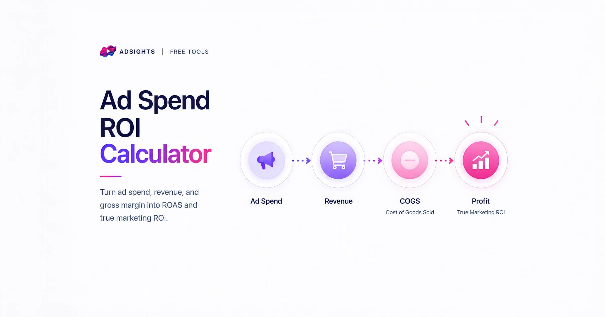
Free ad spend ROI calculator: turn advertising spend, the revenue it drives, and your gross margin into both ROAS and true marketing ROI. See return on ad spend and the COGS-aware, profit-based ROI behind it so you can defend ad budgets with the number finance actually asks for.
Return on Ad Spend (ROAS) is a marketing performance metric that measures the revenue generated per dollar of advertising spend. Unlike ROI which considers all business costs, ROAS specifically evaluates advertising efficiency by comparing directly attributable revenue to ad spend. This metric is crucial for optimizing campaign performance, budget allocation, and overall marketing strategy.
Return on Investment measures the profitability of an investment by comparing the net profit (revenue minus all costs) to the total investment cost. In marketing, it considers all costs including media spend, creative production, technology, overhead, and operational expenses, making it a more comprehensive metric than ROAS which focuses specifically on ad spend.
Incrementality is a scientific measurement approach that determines the true incremental value generated by a marketing activity by comparing outcomes against a statistically valid control group. Unlike basic attribution models, incrementality testing uses randomized controlled trials and sophisticated causal inference techniques to identify what would have happened without the marketing intervention, enabling marketers to understand the real marginal impact of their spending and optimize toward truly incremental growth.
A campaign can return 3× overall while its next $5,000 costs $1,400 in contribution. Test the budget step, margin, and break-even hurdle in an interactive lab.
A campaign can have a healthy average return while its next budget increase destroys contribution. The historical average includes the easier demand you already captured. A scaling decision concerns the demand you can reach with additional spend, at the economics of that additional business.
This is the distinction between average and marginal return. It is also the reason a table sorted by ROAS is not a complete budget-allocation system. Before moving money, you need the relevant response curve, an economic hurdle, and a credible account of how that curve was estimated.
Our MER, ROAS, and nMER guide helps choose the reporting level. This article asks a different question: what would an additional block of spend earn, and would that earning cover its cost? Every numerical result below comes from an explicitly assumed teaching curve, not advertiser data or a recommended spending level.
Average revenue return is total revenue divided by total spend for a defined period and scope. Specify whether the numerator is platform-attributed revenue, total business revenue, or estimated incremental revenue. Those quantities are not interchangeable.
Local marginal return is the slope of a revenue response curve at the current spending level: the change in revenue associated with a very small increase in spend, holding the other modeled conditions fixed.
Finite-increase return is the additional revenue over a proposed budget step divided by that step. A $5,000 increase is not an infinitesimal change. When the curve flattens as spending rises, the return over that block is lower than the slope at its starting point.
Google Meridian distinguishes average ROI, marginal ROI, and response curves in its modeling documentation. Here we use “revenue return” and “ROAS” for revenue-to-spend ratios, then calculate contribution separately. We do not call a revenue multiple a profit margin.
Consider this authored response function for one fixed reporting horizon:
Incremental revenue R(s) = 60,000 × s ÷ (10,000 + s), where s is spend in dollars.
It rises with spend and gradually flattens. Its maximum is $60,000 in the limit. That shape and ceiling are assumptions chosen to explain the arithmetic, not fitted estimates.
At $10,000 of spend, the curve produces $30,000 in incremental revenue: a 3.00× average revenue return. At $15,000, it produces $36,000. The proposed $5,000 increase therefore adds only $6,000 in revenue, a 1.20× return on the increase.
Suppose the contribution margin before advertising is 60%. The extra $6,000 generates $3,600 after the included variable costs but before advertising. Subtract the $5,000 additional spend and contribution falls by $1,400.
| Quantity | Before increase | After increase | | --- | ---: | ---: | | Spend | $10,000 | $15,000 | | Modeled incremental revenue | $30,000 | $36,000 | | Average revenue / spend | 3.00× | 2.40× | | Revenue × 60%, less ad spend | $8,000 | $6,600 |
The campaign remains contribution-positive in total under these assumptions. That does not make this particular increase attractive. “Keep the campaign” and “increase its budget” are different decisions.
Move current spend, proposed increase, and contribution margin independently. The revenue curve stays fixed so you can isolate the effect of each decision input. The dashed segment connects the current and proposed spending levels; its slope is the return over the whole proposed increase.
Select Lower starting spend to try the same $5,000 increase farther up the steep part of the curve. Then choose Higher margin: the original increase earns the same $6,000 of revenue, but at 85% margin it adds $100 in contribution. The curve has not improved. The economics have changed. Open See the budget arithmetic to inspect the endpoints and the local next-dollar return.
This separation matters in practice. Two products can share the same attributed ROAS and have different contribution economics because of fulfillment, returns, discounts, or product cost. Optimizing their budgets against one universal ROAS target can conceal that difference.
Let m be contribution margin before advertising, expressed as a fraction. Let ΔR be incremental revenue caused by the proposed change, and ΔS the additional advertising spend. Under a constant-margin assumption:
Change in contribution = m × ΔR − ΔS.
An increase adds contribution when ΔR ÷ ΔS exceeds 1 ÷ m. At a 60% margin, that revenue hurdle is about 1.67×. At 40%, it is 2.50×. Equality gives zero change in contribution before any additional costs omitted from the model.
Specify the margin calculation. If it includes product cost, payment fees, expected returns, and variable fulfillment, name them. If scaling triggers a new warehouse shift, a production minimum, or another discrete cost, subtract that separately. A constant percentage margin does not represent every operational constraint.
Longer-term customer value can change the numerator, but only if its horizon, retention assumptions, discounting, and cost basis are consistent. Do not compare a lifetime revenue estimate on one side with an immediate cash constraint on the other and call the difference profit.
For the lab’s curve, the local slope is 600,000,000 ÷ (10,000 + s)². At $10,000, it is 1.50×. That is already below the 1.67× hurdle at 60% margin, but it is still higher than the 1.20× earned across the next $5,000.
A common spreadsheet shortcut multiplies the starting marginal return by the entire proposed increase. Here it would forecast $7,500 of extra revenue rather than the curve’s $6,000. It overstates the result because the slope falls throughout the interval.
Use the two endpoints of the response curve for a finite change: R(s + ΔS) − R(s). Reserve the derivative for a genuinely local question. If the model is discrete, compare sufficiently small neighboring budget scenarios and acknowledge the approximation rather than inventing more precision than the model supports.
Real curves require evidence. They may come from randomized budget experiments, geo experiments, or a marketing-mix model with explicit causal assumptions. A scatterplot of weekly spend against weekly sales is not automatically a causal curve: teams often increase spend during promotions or when demand is already strong.
Likewise, a simple before-and-after revenue difference is not necessarily the revenue caused by a budget change. Seasonality, price, distribution, competitor actions, and other channels can move at the same time. Our incrementality-testing guide explains how to design a budget-relevant causal comparison.
Meridian’s documentation notes that response curves hold other channel spending fixed, and that extrapolation risk grows away from the supported spending range. It also discusses how lagged effects complicate short-period return calculations. Those are substantive constraints on interpretation, not footnotes to remove from a presentation.
A curve calibrated during one promotion, creative portfolio, or auction environment may not transfer unchanged. Record the data window, model version, supported spend range, conversion maturity, and treatment definition with every recommendation. Creative improvements can shift the response itself; the lab keeps it fixed only to make the economics inspectable.
Do not build a single precise optimum from an uncertain curve and report it to the dollar. Evaluate a small set of feasible changes. For each, carry the uncertainty in additional revenue through the same contribution calculation, including plausible variation in margin and step costs.
If different credible scenarios imply opposite decisions, quantify the downside and choose how much information is worth buying. A controlled, affordable budget test may be more valuable than immediately committing the full increase. Write down the stopping rule, observation window, and maximum exposure before running it.
Compare alternatives on a consistent basis. A channel with the best local return may have little capacity at that rate; another may absorb a larger block. If changing one channel changes another’s returns, independent one-channel curves are insufficient for the combined move. The relevant decision is the joint change and its total contribution, subject to cash, inventory, and operational constraints.
The conversion-maturity lab adds another practical check: do not estimate the response of a new spending level from an immature cohort and compare it with a fully matured baseline.
Start with the exact proposed action: “Increase spend from X to Y over horizon H.” Define the revenue outcome and whether it is causally incremental. Name the evidence supporting the curve at both endpoints, not just around the historical average.
Show incremental revenue, incremental spend, the contribution-margin definition, any discrete costs, and the resulting contribution change. Include the sensitivity range and the main reason the estimate might fail. Then specify what observation would cause you to hold, reverse, or extend the change.
After the observation window closes, compare the predicted and observed outcomes using the same maturity and attribution definitions. Record surprises as model feedback. Avoid judging the decision solely on whether an uncertain outcome happened to turn out well; evaluate whether the evidence and risk assessment were appropriate when the decision was made.
Average ROAS describes the return across money already spent. Scaling requires an estimate of the next money’s return. Keeping that distinction visible turns a ranking exercise into an economic decision.
Before approving an increase, fill in this five-line memo:
Proposed move: $10,000 → $15,000 over the same reporting horizon.
Additional revenue: $6,000 under the stated response curve.
Economics: $6,000 × 60% margin − $5,000 spend = −$1,400 contribution.
Decision under these assumptions: Hold this increase; the current campaign can still be contribution-positive.
Evidence to revisit: A better-supported response curve, a different budget step, or different contribution economics.
For your account, attach the evidence supporting the revenue estimate and the range of credible outcomes. The ROAS calculator checks the average; this memo checks the proposed change. Neither can establish incrementality from spend and attributed revenue alone.
All amounts are USD in a single hypothetical reporting horizon. The lab assumes incremental revenue R(s) = 60,000s / (10,000 + s), constant contribution margin, and no additional fixed or step costs. It computes the local derivative analytically and the finite-step return from the endpoints. There is no fitted model, uncertainty interval, cross-channel interaction, or recommended budget. The hero is conceptual generated artwork.
The scaling decision: A 3.00× average return does not make the next $5,000 profitable. In this example, the increase earns 1.20× and loses $1,400 after variable costs and ad spend. Test the next budget increase ↓
Illustrative response curve R(s) = 60,000s / (10,000 + s). Increasing spend from $10,000 to $15,000 adds $6,000 incremental revenue. At 60% contribution margin before ads, the $5,000 increase reduces contribution by $1,400.
| Quantity | Default value |
|---|---|
| Average revenue / spend | 3.00× |
| Local next-dollar return | 1.50× |
| Return on $5,000 increase | 1.20× |
| Break-even revenue return at 60% margin | 1.67× |

