Stay Updated
Get the latest insights on creative testing and ad optimization delivered to your inbox.
Get the latest insights on creative testing and ad optimization delivered to your inbox.

Continue reading about this topic with these recommended articles.

A campaign can return 3× overall while its next $5,000 costs $1,400 in contribution. Test the budget step, margin, and break-even hurdle in an interactive lab.

AI-powered marketing tools
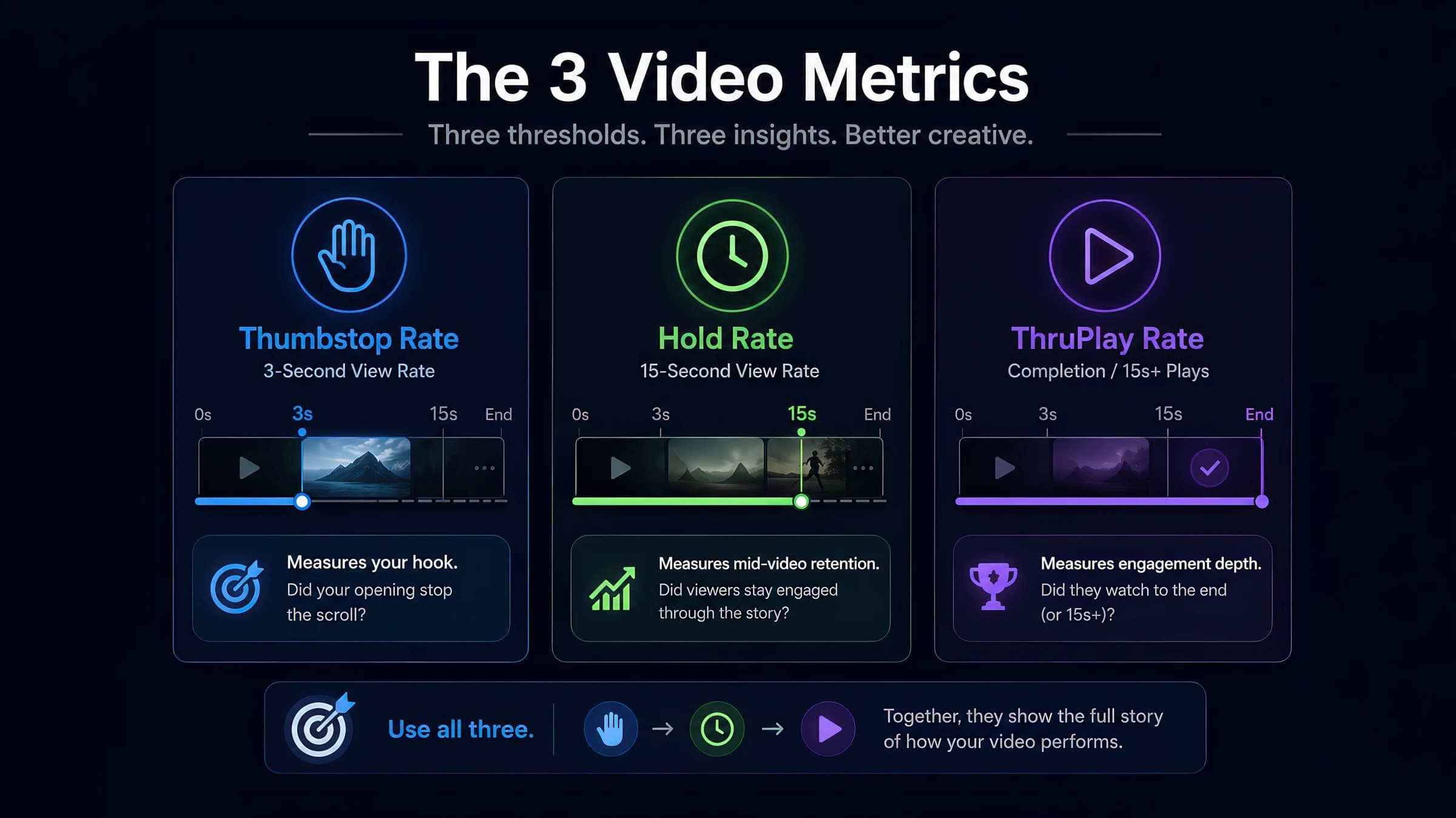
Meta Ads Manager hides the creative diagnostics that matter behind custom columns. This walkthrough shows exactly where to find thumbstop, hold, and ThruPlay — and how to read them without false conclusions.
AI-powered marketing tools
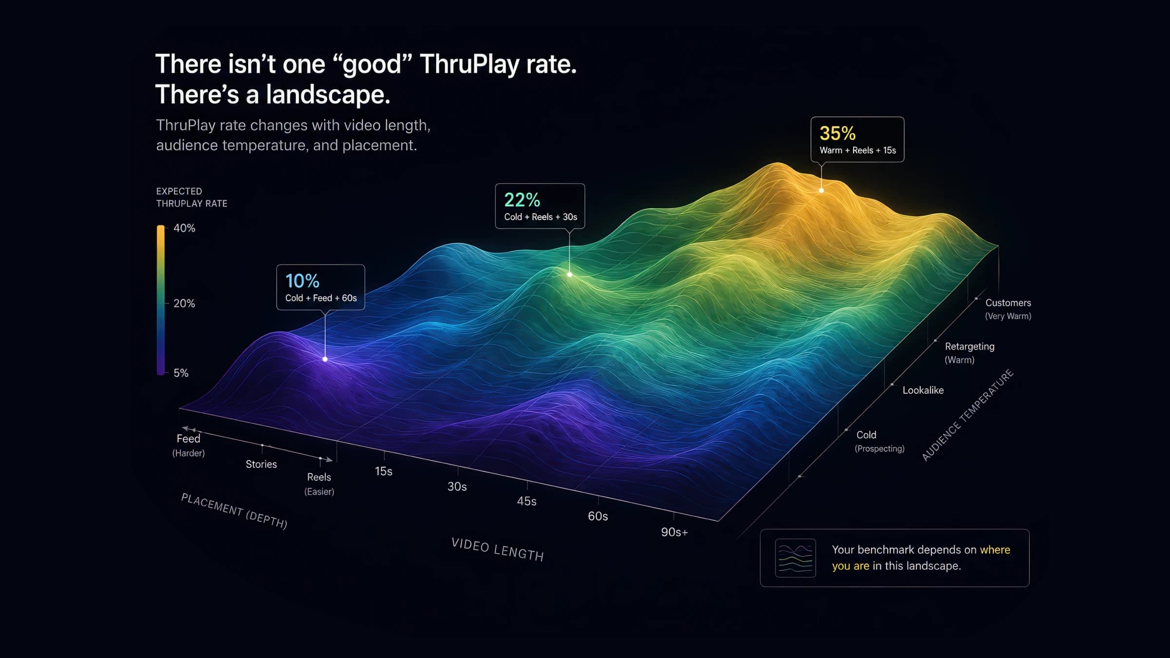
ThruPlay benchmarks shift 10–30 points by video length, placement, and audience temperature. See the full 2026 segmented data — and which number to actually cite.
AI-powered marketing tools

Analyze audience drop-off and retention to find exactly where viewers stop watching your videos. Works for YouTube, Vimeo, TikTok, and Facebook analytics data.

Grade your ad creatives and get actionable recommendations for improvement. This creative quality grader tool evaluates key elements like visual design, messaging, CTAs, accessibility, and platform optimization to help you create high-performing ads across Facebook, Instagram, TikTok, and YouTube. Get detailed scores and personalized tips to optimize your creative strategy.

Calculate Marketing Efficiency Ratio (MER) metrics to evaluate overall marketing performance, attributed efficiency, and new customer acquisition. Use our free MER calculator to apply multiple MER formulas (MER, aMER, nMER), analyze key efficiency metrics, and optimize your marketing ROI with data-driven insights.
Creative fatigue is a quantifiable phenomenon where ad performance metrics (like CTR, conversion rate, or ROAS) deteriorate as target audiences become overexposed to the same creative assets. This decline typically follows a predictable decay curve that accelerates with increased frequency and audience saturation. The impact varies by channel, format, and audience but generally manifests through decreased engagement and increased costs.
Return on Ad Spend (ROAS) is a marketing performance metric that measures the revenue generated per dollar of advertising spend. Unlike ROI which considers all business costs, ROAS specifically evaluates advertising efficiency by comparing directly attributable revenue to ad spend. This metric is crucial for optimizing campaign performance, budget allocation, and overall marketing strategy.
The customer journey maps the comprehensive progression of interactions between a customer and brand across all channels, devices, and time periods. In modern digital marketing, it represents a non-linear, dynamic path encompassing both active and passive touchpoints - from initial brand discovery through consideration, purchase, and ongoing loyalty. This journey requires sophisticated cross-channel tracking, multi-touch attribution modeling, and strategic message orchestration to effectively guide users toward desired outcomes while delivering value at each stage.
A confidence interval provides a range of values that likely contains the true value of a metric, given a certain confidence level. In digital advertising, it helps marketers understand the reliability of their performance measurements and make more informed decisions about campaign optimization. Wider intervals suggest more uncertainty, while narrower intervals indicate more precise estimates of true performance.
Before pausing an ad over rising CPA, check cohort age. Explore how a $50 CPA becomes $30 without an optimization—and when that explanation fails.
Yesterday’s CPA and last month’s CPA may describe cohorts at different stages of completion. Spend can appear before all the conversions associated with it. If you treat the freshest number as final, you can stop a viable creative, misdiagnose fatigue, or credit an intervention for improvement that would have arrived anyway.
The fix is not “always wait seven days.” It is to establish what counts as a cohort, measure how its reporting develops, and compare cohorts at a common age. Then use a clearly labeled projection when the decision cannot wait for complete data.
Google Ads explicitly documents that conversion delay can make CPA appear inflated and ROAS appear depressed. That supports the mechanism, not a universal lag curve. The timing depends on the conversion action, customer journey, reporting pipeline, and account. The numbers in this article are synthetic and should not be reused as benchmarks.
Interaction time is when the advertising interaction occurred. Conversion time is when the customer completed the action. Reporting time is when the action became available in the system you are reading. These timestamps can differ, and not every export exposes all three.
A customer might click on Monday, purchase on Thursday, and have the record imported on Friday. A click-date view can revise Monday’s result after the purchase appears. A conversion-date view can show the purchase on Thursday. Both can be correct while answering different questions.
Before building a maturity adjustment, document which date anchors your report. Also record the conversion window, timezone, conversion action, attribution basis, and whether modeled or subsequently adjusted results are included. “Purchases” is not a complete metric definition.
Google’s Ads API documentation distinguishes conversion reporting fields and available lag segments; availability varies by report. Use those definitions when working with that platform rather than assuming every dashboard date means the same thing.
Imagine a closed click cohort with $3,000 of spend. It ultimately records 100 purchases within the chosen seven-day teaching horizon. At day one, only 40 have appeared. At day two, 60. By day seven, all 100 are present.
| Cohort age | Recorded purchases | Observed CPA | | --- | ---: | ---: | | Day 1 | 40 | $75.00 | | Day 2 | 60 | $50.00 | | Day 3 | 75 | $40.00 | | Day 4 | 84 | $35.71 | | Day 5 | 90 | $33.33 | | Day 6 | 96 | $31.25 | | Day 7 | 100 | $30.00 |
The apparent improvement from $75 to $30 requires no optimization. The spend and the cohort stay fixed; only the recorded outcome count matures. If you had paused the ad at day two and checked again at day seven, the lower CPA would not prove the pause caused anything.
This is why a rolling “last seven days” report can be awkward for diagnosis: it combines cohorts aged roughly one through seven days, each with a different degree of completeness. When daily spend changes, the mixture of immature and mature spend changes too.
Compare Day 2 snapshot with Mature cohort to see CPA fall as purchases arrive. Select Wrong assumption to keep the day-two observations but change the forecast. The sliders let you test the values between those scenarios. Filled bars show what is known at the selected age; dashed bars reveal later observations for this teaching example.
The default day-two example has 60 observed conversions and assumes 60% completeness. Dividing 60 by 0.60 gives 100 projected final conversions; $3,000 divided by 100 gives a $30 projected CPA.
Now change the completeness assumption to 80% while keeping day two selected. The projection becomes 75 conversions and a $40 CPA. At 40% completeness, it becomes 150 conversions and a $20 CPA. The observations did not change. Only your assumption did. That is exactly why the adjusted result must remain labeled estimated.
A useful historical completeness curve follows the same cohort over time. For each sufficiently mature cohort, retain snapshots of the conversion count at ages such as one, two, three, seven, and fourteen days. Choose ages appropriate to the business rather than treating this example’s seven-day endpoint as final for every account.
For an age d, a pooled completeness estimate is:
Conversions visible by age d across selected mature cohorts ÷ their conversions at the chosen mature horizon.
Pooling counts weights cohorts by their mature conversion volume. Averaging each cohort’s completeness ratio instead weights cohorts equally. Those are different estimators; choose intentionally and document which one you use. Avoid letting a cohort with one purchase dominate a daily ratio average.
Use cohorts that are comparable on the dimensions likely to change delay: conversion action, product or purchase cycle, market, device where useful, and relevant reporting configuration. More segmentation trades specificity for stability. If cells become sparse, pool deliberately and widen the uncertainty rather than fitting a noisy curve to every ad.
Keep the snapshots immutable. A report that only exports today’s revised historical totals cannot reconstruct what you knew last Tuesday. Store both the cohort date and snapshot date so backtests can recreate the actual decision.
For a closed cohort, the simple adjustment is:
Projected final conversions = observed conversions ÷ estimated completeness.
Projected CPA = fixed cohort spend ÷ projected final conversions.
For a period containing several cohort ages, adjust each cohort with its corresponding completeness and then sum projected conversions. Divide total spend by that sum. Do not average the daily CPAs, and do not apply one convenient completeness fraction to a period whose spend is heavily concentrated in the newest days.
Zero is a special case. If a recent cohort has zero recorded purchases, this multiplicative method still projects zero. It cannot infer an eventual count from no observed events. Display insufficient evidence rather than a falsely reassuring CPA. A more elaborate model could borrow information from comparable cohorts, but it would introduce additional assumptions that need their own validation.
Adjusting conversion counts also does not automatically adjust revenue. If late purchases have different basket sizes or refund rates, a count-based maturity factor may be inappropriate for ROAS. Build a value-based maturity model if the decision is about value, and define how returns and cancellations enter it.
Take historical cohorts that have already reached your chosen mature horizon. Pretend you are standing at day two. Fit the completeness assumption using earlier mature cohorts, project the held-out cohort, and compare the projection with its eventual result. Roll that process forward through time.
Report signed bias as well as absolute error. A model that consistently understates CPA is dangerous in a different way from a model with symmetric noise. Check error during promotions, tracking changes, unusually large budget increases, and new-product launches rather than judging only an average quiet week.
The lab’s 40–100% slider is a sensitivity analysis, not a confidence interval. An interval for a real forecast must account for observed-count uncertainty and uncertainty in the maturity curve. A historical range can be a useful operational scenario range, but label it honestly rather than attaching a “95%” badge without a statistical procedure.
If old assumptions stop calibrating, suspend the adjustment or broaden the decision range while investigating. A model is not repaired by quietly replacing observed results with its preferred projection.
Conversion lag is one explanation for a recent CPA increase, not a blanket excuse. Check whether the same-age comparison worsened: this Monday’s cohort at day three versus comparable historical cohorts at day three. If the decline persists after matching maturity, the lag explanation is incomplete.
Then inspect the wider system. Did traffic cost change? Did click quality or audience mix change? Was the offer different? Are checkout errors or event-ingestion failures present? If upstream events vanish abruptly, waiting for purchases to mature may delay detection of a broken pipeline.
The creative-fatigue guide covers creative-specific diagnosis. The audience-mix lab addresses composition. Treat these as complementary checks, not competing explanations you choose according to which protects the current campaign.
A practical readout has three views: observed results as of a named snapshot, results for cohorts that meet the maturity cutoff, and projected results for incomplete cohorts. Label all three. State the conversion horizon and configuration version beside them.
Predeclare when an estimate can influence a decision. For example, require the conclusion to remain the same across your documented sensitivity range before making an ordinary budget adjustment. If it crosses your decision threshold, the honest answer may be to gather more evidence. Operational incidents, hard spend caps, or severe losses still need immediate action; a maturity policy should not block incident response.
Assign an owner to reconcile the projection after the cohort matures. Record the original decision, assumptions, later outcome, and model error. That closes the loop between reporting and learning rather than letting yesterday’s estimates disappear when the dashboard backfills.
A recent CPA is a snapshot, not a verdict. Making cohort age explicit lets you act quickly while retaining the distinction between what has happened, what has been reported, and what you expect to arrive.
Use a snapshot like this in the weekly review:
Observed as of day 2: $3,000 spend, 60 purchases, $50 CPA.
Estimated at maturity: $30 CPA, assuming 60% completeness.
Sensitivity: At 40–80% completeness, estimated CPA spans $20–$40.
Next action: If that range crosses our decision threshold, gather more evidence or limit the change. Name who will reconcile the estimate when the cohort matures.
This is an illustrative scenario range, not a confidence interval. For a real readout, use your own backtested completeness range and state the date, conversion definition, and maturity horizon.
The CPA calculator can check spend divided by recorded conversions. It does not adjust for lag; keep that observed calculation separate from the estimate.
The lab uses a fixed $3,000 cohort and authored cumulative counts of 40, 60, 75, 84, 90, 96, and 100. The eventual $30 CPA is known only because the scenario is constructed. It models no refunds, attribution changes, missing events, or uncertainty interval. The hero is conceptual generated artwork. Sources support the reporting mechanisms; the worked example and operating policy are our own.
Before you pause the ad: Compare cohorts at the same age. In this example, a day-two CPA of $50 settles at $30 as purchases arrive. The lab also shows how a wrong completeness assumption distorts the forecast. Explore the cohort clock ↓
Illustrative fixed $3,000 click cohort. At day 2, 60 conversions produce a $50 raw CPA. Assuming 60% completeness gives 100 projected conversions and a $30 adjusted CPA; the projection is not an observation.
| Cohort age | Recorded conversions | Raw CPA |
|---|---|---|
| Day 1 | 40 | $75 |
| Day 2 | 60 | $50 |
| Day 3 | 75 | $40 |
| Day 7 | 100 | $30 |

